Understanding Fully Connected Neural Networks
In the realm of artificial intelligence and machine learning, neural networks stand as the backbone of many modern computational algorithms. Among the various types of neural networks, one of the most fundamental and widely used is the fully connected neural network (FCNN). This article delves into what fully connected neural networks are, how they function, and where they are typically applied.
What is a Fully Connected Neural Network?
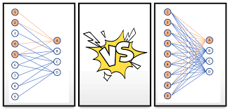
A fully connected neural network is a type of artificial neural network where each neuron in one layer is connected to every neuron in the subsequent layer. Unlike convolutional neural networks (CNNs) that apply convolutional filters and pooling layers, FCNNs consist purely of dense layers without any spatial or temporal subsampling.
The “fully connected” aspect implies that information from every input node is fed to each node in the next layer. This creates a highly flexible architecture that can model complex patterns but at a cost of increased computational requirements and a higher risk of overfitting, especially with large input data.
Structure of Fully Connected Neural Networks
A typical FCNN includes an input layer, several hidden layers, and an output layer:
- Input Layer: The first layer that receives the input signal to be processed.
- Hidden Layers: One or more layers where computation and transformation occur. Each neuron here applies a weighted sum on its inputs followed by a non-linear activation function.
- Output Layer: The final layer that produces the output for given tasks such as classification or regression. The number of neurons in this layer corresponds to the number of output classes or values.
How Does it Work?
The core operation within an FCNN involves matrix multiplication between inputs and weights, addition with biases, followed by an application of an activation function like ReLU (Rectified Linear Unit) or Sigmoid. These steps can be summarized as follows:
- The input data is presented to the input layer.
- The data travels through hidden layers where neurons apply weights to inputs, add biases, and pass them through activation functions for non-linear transformations.
- This process repeats across all hidden layers until reaching the output layer.
- In classification tasks, a softmax activation function may be used at the output layer to generate probabilities for different classes.
Training Fully Connected Neural Networks
To train an FCNN, backpropagation with gradient descent is commonly used. During training:
- The network makes predictions based on current weights.
- An error metric or loss function evaluates how well these predictions match actual targets.
- The gradient of this loss with respect to each weight is calculated using backpropagation—essentially determining how changes in weights affect overall error.
- Weights are then adjusted in the direction that minimizes this error using gradient descent or its variants like Adam optimizer.
Applications of Fully Connected Neural Networks
Fully connected neural networks are versatile and have been applied across various domains such as:
- Digital Recognition: Recognizing handwritten digits or characters using datasets like MNIST where spatial relationships between pixels are less critical than patterns recognized by dense connections.
- Predictive Analytics: Forecasting future trends based on historical data across finance, weather prediction, etc., where complex relationships between data points must be learned deeply.
- Natural Language Processing (NLP): Though recurrent neural networks (RNNs) and transformers have become more popular for NLP tasks due to their ability to handle sequences better than FCNNs can still play roles in simpler text classification problems when combined with proper text representation techniques like TF-IDF vectors.
Limits and Considerations
Fully connected networks tend to require more parameters than other architectures such as CNNs for similar tasks due to their lack of parameter sharing. This increases memory requirements and computational costs while also making them prone to overfitting—especially when dealing with high-dimensional data like images. Regularization techniques such as dropout can help mitigate overfitting by randomly disabling neurons during training which encourages redundancy within the network architecture ensuring no single set of neurons becomes too critical during inference time thereby improving generalization capabilities on unseen data sets.
In conclusion fully connected neural networks though not always optimal for every machine learning task remain foundational tools within AI researcher’s toolkit due understanding their straightforward structure ease implementation they provide excellent baseline models against which newer more complex architectures can compared improved upon future advancements field continue evolve develop.”

